Power Query and the Abyss

I stared into the abyss of this business challenge. The old method consisted of 200+ odd ball queries in an Access database. No documentation. You know how it happened. Years ago some hack fixed a small problem with a few queries when the business challenge was small. The business grew in size and complexity, more hacks by other hackers and now: 200+ odd ball queries limp along doing a barely adequate job of what is now a potentially costly business process. By the way the old process took about 5 man days and was fraught with error. Auditors nightmare & a beast to support. There had to be a better way.

My gut feel was that Power Query had potential to “help” but I can honestly say I had no clear vision of the solution when I dove in. ***Spoiler alert*** Power Query not only helped, it turned out to be THE solution. Such a slick solution I felt motivated to blog about it. I’ll dumb down the actual story, but to appreciate the “power” in Power Query one must appreciate the challenge.

Think of a large distributor of hard goods that had negotiated special rebate terms with its best customers. CustomerA gets 8% rebate on hand tools purchased in the Midwest, CustomerB gets 7% rebate on all products purchased in the West, CustomerB also gets 6% rebate on Plumbing parts purchased in the Southeast which were manufactured by CompanyZ… and the list goes on. All these unique terms are captured & updated monthly by the Contracts department in a single spreadsheet. Of course this is a sacred spreadsheet that can only be viewed – thus these terms must be extracted “as is”. Here is a dumbed down sample of the controlling table “RebateMaster” found in the spreadsheet:

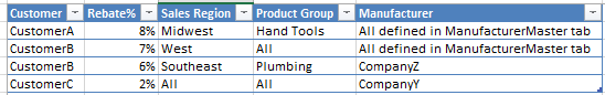
The more I looked at this table the darker the abyss became. How to apply these rebate rules to the Sales data to derive the records that meet this crazy criteria? I’ll skip the details of the dead ends explored. The ray of hope started to shine when I thought of this as more of a “layered filtering” or “funnel” challenge. Looking at the columns from left to right, each column further filters the overall sales dataset by some criteria. If for every row in this table I could start with all the sales data and filter by [Customer], then filter that result by [Sales Region], then filter that result by [Product Group], then [Product List], then [Manufacturer]… the result would be all the sales records that meet the criteria for that rebate record. Eureka!!! That’s the data we seek!!!

How can Power Query do this “funnel”? With a paradigm shift – well it was a paradigm shift for me. My experience with Power Query to date was limited to traditional data cleansing and shaping at the detail record level. This challenge was far from traditional. My paradigm shift: Stay at the rebate table level and process whole tables worth of Sales data with M code. This is really much easier than it sounds.

Following best practices recommended by Ken Puls I knew to create a connection only queries to my data sources. For brevity… trust me that I created

• srcRebateMaster_tblCustomers – table of customers that get rebates
• srcRebateMaster_tblMfg – table of manufacturers that participate in the rebates
• srcSales – table of Sales data pulled from SQL server. Since this query uses some Ken Puls’ trickery (but a bit off topic) I include it below

Time to bring in the Rebate table shown above. No tricks here, just pull it in like any ole Excel table. Now the paradigm shift. Add a custom column [SalesThisCustMfg] that filters srcSales by [Customer] & [Manufacturer]. Then add a custom column [SalesThisRegion] that filters [SalesThisCustMfg] by [Sales Region]. Likewise for [SalesThisProductGrp]:

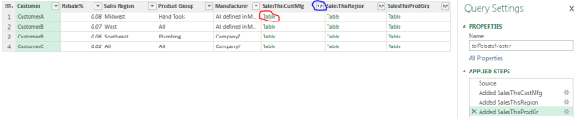
Later I will show the M code for these Added Columns. First a little refresher on the Power Query interface. If I were to click on “Table” circled in red I would see the sales records for CustomerA. If instead I were to click on the funky arrows circled in blue I would see the sales records for all the customers in the table. Now that is powerful!!! Love this feature!!! This is very handy place to prove out the formulas and troubleshoot issues ongoing. Thus I will not add any more steps to this query, but rather save it as is (connection only) so I can reference it for the final processing steps in another query and also have it readily available for debugging down the road.

To continue, from the list of queries, right click on the query tblRebateMaster and select “Reference”. This creates a new query where the source is defined as tblRebateMaster and we are right where we left off. Good news is most of the work is done. The quick finish is to remove all but [Rebate%] and [SalesThisProdList] (remember it was the last filter applied in our funnel), then click those funky arrows on [SalesThisProdList] to get the result set of Sales records we were after. Add another Column which multiplies [Rebate%] by [Sales Amount] and you have now calculated the [Rebate Amount]. Close and load this to your data model and pivot away on your newly defined Rebate data.

Bask in the glory of replacing 200+ SQL queries!!! Now those folks in Contracts can add/remove customers as needed. Yes, I might need to update some of the “funnel filters” if a rouge salesman negotiates a completely new rebate term – but with Power Query I’m not scared…

Oh yeah, there is that matter of the M code that does the “funnel filters”. Here tis:

[SalesThisCustMfg] – needs to filter srcSales by [Customer] and [Manufacturer]. Assumes srcSales fields of [Cust] and [Mfg]. Note – There is a limitation that the field [Customer] cannot be referenced inside Table.SelectRows(). Solution is to first assign the value of [Customer] to the variable ThisCustomer, which CAN BE referenced inside the function. Same for [Manufacturer].

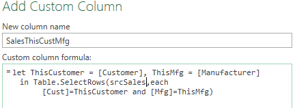
[SalesThisRegion] – needs to filter [SalesThisCustMfg] by [Sales Region]. Assumes srcSales field of [Sales_Region]

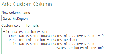
[SalesThisProdGrp] – needs to filter [SalesThisRegion] by [Product Group]. Assumes srcSales field of [Prod_Grp]

srcSales: Instead of just pointing the query at the whole Sales table, for performance I pulled only the Sales records for the Customers and Manufacturers that participate in the rebate program.  Here is the M code (paraphrased):

srcSales:
FiscalStart = fnGetParameter(“FiscalStart”),
FiscalEnd = fnGetParameter(“FiscalEnd”),
CustList = Table.Column(srcRebateMaster_tblCustomers,”Customer Number”),
CustListSQL = “‘” & List.Accumulate(CustList, “”, (state, current) => if state = “” then current else state & “‘,'” & current) & “‘”,
MfgList = Table.Column(srcRebateMaster_tblMfg,”Manufacturer”),
MfgListSQL = “‘” & List.Accumulate(MfgList, “”, (state, current) => if state = “” then current else state & “‘,'” & current) & “‘”,
SQL=”Select * from Sales
where Customer in (” & CustListSQL & “)
and Manufacturer in (” & MfgListSQL & “)
and Fiscal_Period between ” & FiscalStart & ” and ” & FiscalEnd,
Source = Sql.Database(“server1.myco.com”, “Sales”, [Query=SQL]),

srcSales Notes:

• FiscalStart/FiscalEnd are pulled from a parameter table like Ken blogged

• CustList/MfgList are tables in the Excel file referenced by srcRebateMaster

• CustListSQL/MfgListSQL – same data as above, but reformatted from a table to a delimited string compatible with SQL

• SQL – string of executable SQL built using above parms, which is then used in Sql.Database()

As a final note I will add that I was concerned about performance during development. In my real rebate dataset I have roughly 10 “funnel filters”, hundreds of customers that get rebates, and 10 million Sales records of which 10% get some kind of rebate. I toyed a bit with Table.Buffer() and I pondered query folding… Truth is performance never was a problem. My data model loads in less than 5 minutes which serves the need well.

I hope you find this info useful. Perhaps next time you find yourself staring into the abyss, Power Query will be your ray of hope…

 

Pivots & PowerPivot Don’t Mix…. Or Do They ???

I was recently faced with a challenge:

CxO: Your PowerPivot dashboard is awesome! But… it is too big to email to the Regions… and they don’t need to see each other’s data…

Me: Sir we have many ways to securely disseminate this data to the field. The Microsoft BI stack… On premises… Cloud… SharePoint… licensing… $$$…

CxO: <eyes glazed over> just send them an email attachment…. only their data… preferably today… then monthly…

Yes, old school email reporting is alive and well in Corporate America. Much as I love all the new possibilities (thinking animated bubble chart of near time data on an iPad… screencasted to a 4G display… I digress…), when the field needs a table of data we still need to get them that table – as they want it, typically email. Many platforms do this and do it well (thinking SSRS), but if you just built a management dashboard in PowerPivot and you want the field’s data to match, it’s best to produce the field’s data as a derivative of the dashboard. I’ll pause here for questions…. Good… glad we agree.

So that’s the “why”. Fortunately the “how” is pretty easy. I hope to make your experience even easier by sharing my methods here. I don’t pretend any of this is new or cutting edge, but as I had to seek out many answers from many places… I’m hoping this collection will be of value.

General Approach:

• Crunch the data in PowerPivot: Premise here is that a PowerPivot dashboard has already been built. Many have blogged about this. Great examples abound. PowerPivot rocks!!!
• Expose the PowerPivot data as a table in Excel: It’s a simple DAX query, but as it is a bit of an unusual approach the steps are detailed below.
• Pivot on that table into another spreadsheet: Old school Excel Pivot method that should not be forgotten. Details revisited below.
• Distribute: email. ‘nuf said.

Expose the PowerPivot data as a table Excel:

Most of the time in the PowerPivot world we create PowerPivot tables and PowerPivot charts to see the data in Excel. Works great most of the time. However PowerPivot tables do not behave like regular tables. In this case it is a real bummer that a PowerPivot table can’t be the data source for a regular Pivot Table. Fortunately, we can expose the PowerPivot data via a DAX query that results in an Excel table that behaves like a regular Excel table. To illustrate, consider a simple PowerPivot data model of an Expense table and a Date table. From a clean sheet in Excel select Data/ExistingConnections/Tables and select the Expense table then Open. You should now have an exact copy of PowerPivot’s Expense table as a table in Excel, in this case named Table_Expense. The good news is this table can be used as a data source for a traditional Excel Pivot Table. Yeah!

PowerPivot Data Model:

Bring PowerPivot Table into Excel:

Expense Table in Excel:

True to our premise though, we need to limit this data by Region so each Region gets only their data. Right click on the table and select Table/EditDax. You have now entered the brave new world of DAX where possibilities are limited only by your imagination and skill. Careers can be made by those who dive deep into DAX… powerful stuff… Truthfully, my DAX skillset is limited to just pulling desired fields with perhaps a simple filter or two – which is all we need for this project. For this illustration I created the following DAX query:

DAX Query example:

For me DAX syntax is a bit odd, but manageable. In laymen’s terms we Summarize the Expense table, pulling the fields listed and filtering by Region=1 and Year=2014. Note that you can pull a field from related tables such as DateDim[FiscalMonth]. Also note that filters must be fully specified with the table name such as Expense[Region]=”1″. That my friends is probably enough DAX knowledge to satisfy most of your DAX needs. You are welcome. With the curtain falling on Act I, here is the filtered Expense table in Excel:

Expense Table Filtered for Region 1:

Pivot on that table into another spreadsheet

Bravo!!! Act I was marvelous. We begin Act II with a beautiful table of data that we can treat like a traditional Excel table. We can Pivot on Table_Expenses into a spreadsheet in another workbook. Open a clean new workbook and select Insert/PivotTable. Define the data source as in my example C:\temp\ExpensePP.xlsx!Table_Expense.

Create a traditional Pivot Table:

Here is a simple pivot showing summarized data for Region=1:

Note that the ExpenseByRegion workbook shown is a simple old school Excel workbook with an old school Pivot Table with the pivot’s data loaded in the Pivot Cache. To see the contents of the Pivot Cache, drill on the Grand Total. You will see the detail records for Region 1 and only Region 1. This is a very efficient report to email as it contains one copy of the detail Expense records for Region, yet the report consumers can drill to the detail as needed. In my real world job I have a PowerPivot Dashboard that is over 80MB, yet it spawns 5MB derivative reports for each Region that can easily be emailed. After the Region 1 report is created, I modify the DAX for Regions 2-4, refreshing the ExpensesByRegion workbook each time to create region specific workbooks.

With this approach I satisfied the immediate need & survived another day. But what about the next month??? Must I redo all this??? What about that big ugly sheet I created in my beautiful Dashboard workbook… Are my Dashboard users stuck with that too??? Well, for my grand final & encore:

As a final step I “hack the DAX” to prevent the table from populating so it won’t unnecessarily bloat my Dashboard, and then hide the sheet so as to not confuse my Dashboard users. What is that DAX hack? For me & mine I insert a bogus filter that results in an empty table. I could just delete the sheet (including Table_Expense) & recreate it next month, but this way the DAX query (which I don’t want to recreate, or go find elsewhere) stays intact, easy to modify.

DAX which forces an empty table:

So next month I refresh the Dashboard, unhide the Sheet with Table_Expense & modify the DAX for each Region, refresh the ExpenseByRegion workbooks. Rinse… Repeat…

Editing the DAX too manual you say??? I agree, and hope to find a method to programmatically control the DAX someday… But back to the real world – those Regional folks are a bit picky and demand their own unique reports. This manual step of editing the DAX is where some of that uniqueness is addressed. Automation good. Agility sometimes better.

Hope this helps. I also hope to hear suggestions from others. Till then… Pivot Onward… PowerPivot Onward… and when necessary do both!!!

OneDrive – My Gal Again

OneDrive – My Gal Again

Perhaps you think I am coming late to the OneDrive party. Actually I came early, and have finally returned. Years ago I “dated” Microsoft Mesh (a part of Windows Live) and felt jilted when her guardian (Microsoft) ended our relationship by taking her off the market. I tried others (Dropbox, Zoho, Google…) but no spark, no zeal, and my Customers typically blocked them at the firewall. Well, time heals all wounds, hardware/software never stand still, and customers evolve. These things fell into place: SkyDrive becomes OneDrive, Corporate America adopts Office365 (which includes 1TB OneDrive for Business), Solid State Drives become affordable, and the OneDrive Sync feature matures. SHAZAM! The old girlfriend is back, cuter than ever and I’m desperately seeking a long term relationship. I’m giddy for her all over again.

Seriously, OneDrive Sync could not have come at a better time for me. I spend most of my day pulling data, mashing data, posting data, repeat. It’s more glamourous than it sounds because I use smoking hot tools like PowerPivot & Power Query, but the drudgery of managing the files does get me down. This is further complicated by the fact the pulling/posting often involves other PCs with special applications and security. Then there is my “workhorse” laptop that does most of the ETL & reporting magic (via large memory & Solid State Drive). I needed help keeping my source files, ETL files, and my PowerPivot files in sync across all these devices. OneDrive Sync lets me do just that.

Now the nitty-gritty. Like all my other girlfriends, OneDrive & Sync are not perfect. Beyond the cute smile, fancy clothes, and sweet perfume there are a few less attractive features to this beauty. Frankly if I were not able to deal with them, this relationship would have never made it past the first date.

Challenge #1) You can only sync data that is stored in your Windows User directory (i.e. C:\Users\JohnDoe\OneDrive for Business). So in my case, ETL processes that feed PowerPivot are hard coded to a specific path such as C:\Data – this is a huge problem. I can’t feasibly change all my code, and even if I could the paths would not be consistent as I use different User IDs on different devices.

Solution #1) Move the data to the sync folder, then create a symbolic link to that location. For me it was as simple as dropping to a Command Prompt and running the old DOS Command:
mklink /d c:\Data “C:\Users\JohnDoe\OneDrive for Business\Data”

Note the quotes around the destination path are required since the path has spaces.

Now when my ETL & PowerPivot processes look for data at C:\data they get redirected to the OneDrive synced folder. No changes required for any of my applications/scripts/data models/etc. I do suggest you review your device’s backup strategy to make sure it properly handles this setup – but that’s another topic.

Challenge #2) Excel is too dang smart. When you have Excel save a workbook to the OneDrive synced folder it knows there is a SharePoint server in the mix (OneDrive) and Excel will not only write to the local drive, but it will also write to SharePoint. WHAT??? To make matters worse, you can’t turn this Excel “feature” off. WHAT WHAT??? Yes, I was a bit surprised by this too. You hardly notice it if the file is small and your path to the SharePoint server is fast – but I’m talking about OneDrive (SharePoint in the cloud) and large PowerPivot files… painful slow… makes my Solid State Drive seem slower than a 1980’s floppy drive…

Solution #2) Use the Symbolic Link you created for Challenge #1. You see if Excel saves the workbook to the path C:\Users\OneDrive for Business\Data\ then Excel sees SharePoint and insists on saving to it – BUT – if Excel saves the workbook to the path C:\Data\ it is not smart enough to realize SharePoint is in the mix and it will behave normally. Gotta love it when 1 fix works for 2 problems.

I’ll also mention here that UNC paths fool Excel also. So if for some reason you choose not to use the symbolic path shown above you can specify the path to save your workbooks as \\<device name>\Users\JohnDoe\OneDrive for Business\Data and Excel will not notice SharePoint.

So here I am in a newly re-committed relationship with the ole gal (OneDrive for Business with Sync). At this point my gal is syncing over 1,000 files that amount to over 40GB of data. Of that about 1 to 10GB is updated daily and my gal ain’t complaining. Nothing like a love story with a happy ending.

A few other notes/references:

“OneDrive” is the consumer version. “OneDrive for Business” is the commercial version available in Office 365. All references to OneDrive in my comments here refer to “OneDrive for Business”. I have only casually used the consumer OneDrive and probably won’t until Microsoft integrates the two with a single client.

OneDrive is surely due to mature in the coming months. The challenges/solutions discussed here may be moot very soon. Stay tuned.

The setup/configuration/usage of OneDrive for Business is easy and well documented in many places such as here… here… and here… No need to repeat in this blog.

I have not tested, but I suspect the solutions described here will disable any multi-user edit functions in Excel.

Though I often kid about my “girlfriends”, I should clarify that I’m happily married and otherwise fully occupied working out the bugs in that relationship.

PowerPivot – CSVs “The SQL Way”

Despite all the technology at our disposal today, when it comes to exchanging data between systems – text files are still the king. The venerable CSV file format is still the least common denominator in the import/export of data. The good news is the Microsoft Excel/PowerPivot/PowerBI stack is a very efficient tool for crunching CSV data into state of the art Charts/Tables/KPIs/Dashboards/etc. However, real world challenges (like dirty data) often turn what should be a straight forward process into a series of speed bumps, hurdles and sometimes dead ends. Described here are some of the tricks/techniques I use on a daily basis to process CSV data with the Microsoft BI tools.

There are many ways to process CSV files. If you are looking to import just a few simple files on an ad-hoc basis there are several methods more simple than The SQL Way I share here. However, if you are tasked with building a process that is robust, repeatable and easily supported… then read on…

Why I do it The SQL Way:

• Dynamic! With SQL in my ETL path I can quickly make changes to meet the dynamic demands of my data consumers
• Documentation! Sometimes I push out very important data sets (think litigation) and by providing the SQL used in the ETL it goes a long way to explain where the data came from and how it was compiled. (Same for DAX by the way)
• Performance! By doing some of the ETL work in the SQL on import, I can keep my tables smaller, perhaps summarized or preprocessed. Keeps the load time and memory requirements down for my data consumers.

Assumptions:

• You have little to no control over the format of the source data. It is given to you in CSV format (which at best is loosely defined standard often misused). It is given to you periodically and your goal is to import the data into PowerPivot so it may be combined with other data and visualized in Pivots and Charts.
• The project is not well defined, thus you can expect many changes in source data and desired visualizations. Somebody is going to move your cheese. Count on it.
• Source data files may need to be combined to form a single table in PowerPivot (such as sales from different regions, different reporting periods, etc…)
• Source data files may need to be joined or filtered to form a single table in PowerPivot (such as importing sales data for only those customers that exist in a separate file)

Approach:

• Build a Schema.ini file that describes the CSV source data
• Define PowerPivot Connection to the source CSV files
• Create the SQL necessary to extract/filter/transform the source data into a PowerPivot data model
• Create DAX defined columns and measures as needed (not described here)
• Create additional dimensions as needed (not described here)
• Create desired visualizations in the way of Pivot Tables and Charts (not described here)

Build a Schema.ini file:

The bad news is the Schema.ini file format is NOT well defined. I found a few gems on Internet forums that helped me clear hurdles, but I never found a comprehensive resource. The good news is Excel provides a decent Wizard that does most of the heavy lifting. Follow along closely as these steps are not all that obvious.

1. Open a new spreadsheet in Excel (2010 version for this example). On the Data Ribbon select to Get External Data, From Other Sources, From Microsoft Query
2. From the Choose Data Source panel, select <New Data Source>
3. From the Create New Data Source pane, give a bogus name (really does not matter), Select the driver “Microsoft Text Driver(*.txt,*.csv)”, click the Connect button
4. From the ODBC Text Setup pane select the proper directory for your source CSV file, click the Options button
5. Still from the ODBC Text Setup pane click the Define Format button
6. From the Define Text Format pane select the source CSV file, and set the Column Name Header /  Format: / Delimiter:  fields to match your source CSV file
7. Still from the Define Text Format Pane you now get to enjoy the magic… click the Guess button and then the OK button. Ignore any error message you get at this point and back all the way out of the Wizard and even close the spreadsheet – for at this point you have accomplished your goal… you have created the Schema.ini file!!!
8. Edit the schema.ini file with your favorite text editor and make adjustments per notes below.

Schema.ini Notes:

• the schema.ini file must reside in the same directory as the source CSV file
• if you use the Wizard to create the schema.ini file, it will contain entries for all files found in the directory. To keep the schema.ini clean, I typically keep each report type in its own directory. c:\data\report1 has a schema.ini that defines report1.csv; c:\data\report2 has a schema.ini that defines report2.csv; etc…
• As a general rule, I define all columns in the schema.ini as “Char Width 255” & let PowerPivot convert the fields to the desired data type. All hail PowerPivot and its ability to change data types on the fly!!!
• Dates in source CSV data can be problematic. Most times you can define in Schema.ini the date fields as “Char Width 255” and in PowerPivot as “Date”. However depending on the format of the source data you may need to specify something like DateTimeFormat=”d-mmm-yy hh:nn:ss” in the schema.ini file in order to help PowerPivot with the transform. One limitation to note – schema.ini assumes all dates in a given source file are of the same format. If that is not true in your case, define in schema.ini the date fields at “Char Width 255” and in PowerPivot as “Text”, then sharpen up your DAX skills to create a defined column of type “Date”.
• PowerPivot can handle “dirty” column names most of the time. It will often just drop the offending character. However I found on occasion PowerPivot will lock up on the import if the column name is too weird. In such cases I can often edit the schema.ini file and remove the offending character from the column definition.
• If the source CSV data contains control characters (other than Carriage Return, Line Feed, End of File, etc) the results can be unpredictable. I have had cases where a text file would only partially load (with no error message thrown) because the 026 control character was somehow embedded in a user input text field. Thus I typically scrub the CSV file before import to remove extraneous junk. On an ad-hoc basis I use NotePad++ to search/replace. For more complex or systematic processes I depend on a PowerShell script that cleanses the files before import. I also use PowerShell to perform many other ETL functions, but that is a whole other topic 🙂
• Depending on how your source CSV file treats text delimiters, you may find this schema.ini setting to be handy: textdelimiter=none. This is another of those under-documented settings that has saved me much grief.

Define the PowerPivot Connection & Import first Report:

1. From the PowerPivot Window (Excel 2010 64 bit for this example), Home Ribbon, select to Get External Data From Other Sources
2. From the Table Import Wizard panel select “Others (OLEDB/ODBC)”
3. From the Connection String panel, define a useful name for the connection (such as “CSV Files via SQL”) and click the Build button
4. From the Data Link Properties panel, Provider tab, select “Microsoft OLE DB Provider for ODBC Drivers” and click the Next button
5. Still from the Data Link Properties panel, Connection tab, select “Use Connection String” and click the related Build button
6. From the Select Data Source panel, give a DSN Name such as “report64” and click the New button
7. From the Create New Data Source panel select the “Microsoft Access Text Driver (*.txt, *.csv) and click the Next button
8. From the Create New Data Source panel browse to the desired location such as c:\data and give a suitable file name such as Report64 and click Next and then click Finish
9. From the ODBC Text Setup panel select OK (assuming you have already created the schema.ini file described above)
10. From the Data Link Properties panel (again) select the OK button
11. From the Table Import Wizard panel (again) verify the connection string looks something like the following and click Next:
    Provider=MSDASQL.1;Persist Security Info=False;Extended Properties=”DBQ=C:\Data\Report1;DefaultDir=C:\Data\Report1;Driver={Microsoft Access Text Driver(*.txt,*.csv)}; DriverId=27; Extensions=txt,csv,tab,asc; FIL=text; FILEDSN=C:\data\report64.dsn; MaxBufferSize=2048; MaxScanRows=25; PageTimeout=5; SafeTransactions=0;Threads=3;UID=admin;UserCommitSync=Yes;”
12. From the How to Choose the Import Data panel, select to Write a Query and click the Next button.
13. From the Specify a SQL Query panel, define a useful name and the following as a SQL Statement and click the Finish button:
    select * from c:\data\report1\report1.txt
14. Data should now be imported to a PowerPivot table. Check/set the Data Type for each column & refresh to ensure PowerPivot can handle the desired transforms.

Import subsequent CSV reports:

1. From the PowerPivot Window, Design Ribbon, select Existing Connections
2. From the Existing Connections panel, select to Open the “CSV Files Via SQL” connection just created.
3. As above, specify the desired table name and SQL query for the next report and click Finish
4. As above check/set the column data types and refresh…

PowerPivot Connection & Import Notes:

• Only 1 PowerPivot connection needs to be defined. You can import all your CSV tables via this connection assuming your SQL query fully specifies the file path. Note that you can use UNC style file paths in the SQL query (\\<sharename>\data\report1\report1.txt as an example).
• I have NOT figured out how to use environment variables or the like to make the SQL queries somewhat dynamic. At this point all my SQL queries are static. I am truly open to suggestions here. Large projects can result in *many* static queries that ultimately need to be modified.

SQL Notes:

• the SQL functionality is limited by the Jet database (aka Microsoft Access). Tis not as good as T-SQL, but not too bad. Syntax is often the challenge, but most is well defined in various Internet forums.
• When you need to combine multiple CSV source files into a single table use the Union All command. For example:
  select * from c:\data\SalesReports\2011full.csv
  union all
  select * from c:\data\SalesReports\2012full.csv
  union all
  select * from c:\data\SalesReports\2013ytd.csv
• When you need to limit the records by another file, use a join such as:
  select *
  from c:\data\SalesReports\2013ytd.csv s, c:\data\Customers\CustListA c
  where s.custno=c.custno

Credits:

I beg forgiveness for not properly acknowledging those that I have learned from. It has been a long and winding path to this point and alas I have not taken good notes. The best can do at this point is call out those who I sponge from regularly:

• www.powerpivotpro.com (Rob Collie)
• www.ssas-info.com/VidasMatelisBlog  (Vida Matelis)
• www.mrexcel.com  (Bill Jelen)
• www.powerpivotblog.nl  (Kasper de Jonge)
• www.sqlblog.com/blogs/marco_russo   (Marco Russo)
• www.denglishbi.wordpress.com  (Denny English)

Update 1/18/2014 – For a little more detail on the process of creating the schema.ini file, including screen shots, see Teo Lachev’s blog: http://prologika.com/CS/blogs/blog/archive/2014/01/17/auto-generating-schema-ini.aspx

Update 10/3/2014 – Hit a snag today. Tried to import a CSV file that had a dash “-” in the file name. Import routine did NOT like the dash. I tried various bracketing methods including `'[] to no avail. Ended up changing the file name using underscore “_” instead of dash. Just thought I’d share…

Update 3/25/2015 – Again had a challenge with a – in a file name. I was able to fix the issue using the character ` (found on the tilde ~ key on my keyboard). Trick is to tic the start of the path to the last \, then tic after the last \ to the end of the path. Example:
select * from `c:\somedir\anotherdir`\`some-file.txt`

Update 4/2016 – Again I had a challenge with a file name – but this time with an Excel file on a Windows Share where the share name had dashes and dollar signs. Excel file??? Yes, I use this same approach to read Excel files via CSV. Just pick the “Microsoft Excel Driver” instead of the “Microsoft Access Text Driver” described above. Anyway back to this path issue… the solution: square brackets
Example for an Excel file:
select * from [\\servername\sharename\somedir\some-file.xlsx].[sheetname]

Update 10/2019 – My how times have changed – but some things not so much. I got a nice “thank you” today from a reader that reminded me this old post is still relevant. Grateful I am for the kudos, but I am now compelled to confess I haven’t used the “SQL Way” method discussed here in several years. A few years back Power Query matured into a very robust data manipulation and ETL tool. I use it exclusively. There now… the truth has set me free to Power Query onward…

Why do I keep making updates to this old blog? For MY future reference of course…